CNNs Demystified: From Image Recognition to ECG Analysis

Published on April 18, 2025 | 12 min read

As a Senior Chief AI Engineer at Samsung R&D, I’ve spent the last few years working at the intersection of machine learning and human health. From improving smartphone vision systems to decoding heartbeats, I’ve seen Convolutional Neural Networks (CNNs) evolve into powerful tools beyond just image recognition.

In this blog, I’ll unravel the “why” behind CNNs, show you how they preserve meaningful structure in data, and share how we’re adapting them to save lives—one heartbeat at a time.

The CNN Advantage: Preserving Spatial Relationships

Imagine trying to understand a sentence after randomly shuffling its words—that’s what traditional neural networks do to images. Flattening a 256×256 MRI scan into a 1D vector throws away the spatial relationships that matter most.

            # Problem: Flattening a 256×256 MRI scan
            flattened = image.reshape(1, 256*256*3) # 196,608 features!
            # Loses all spatial context between pixels
        

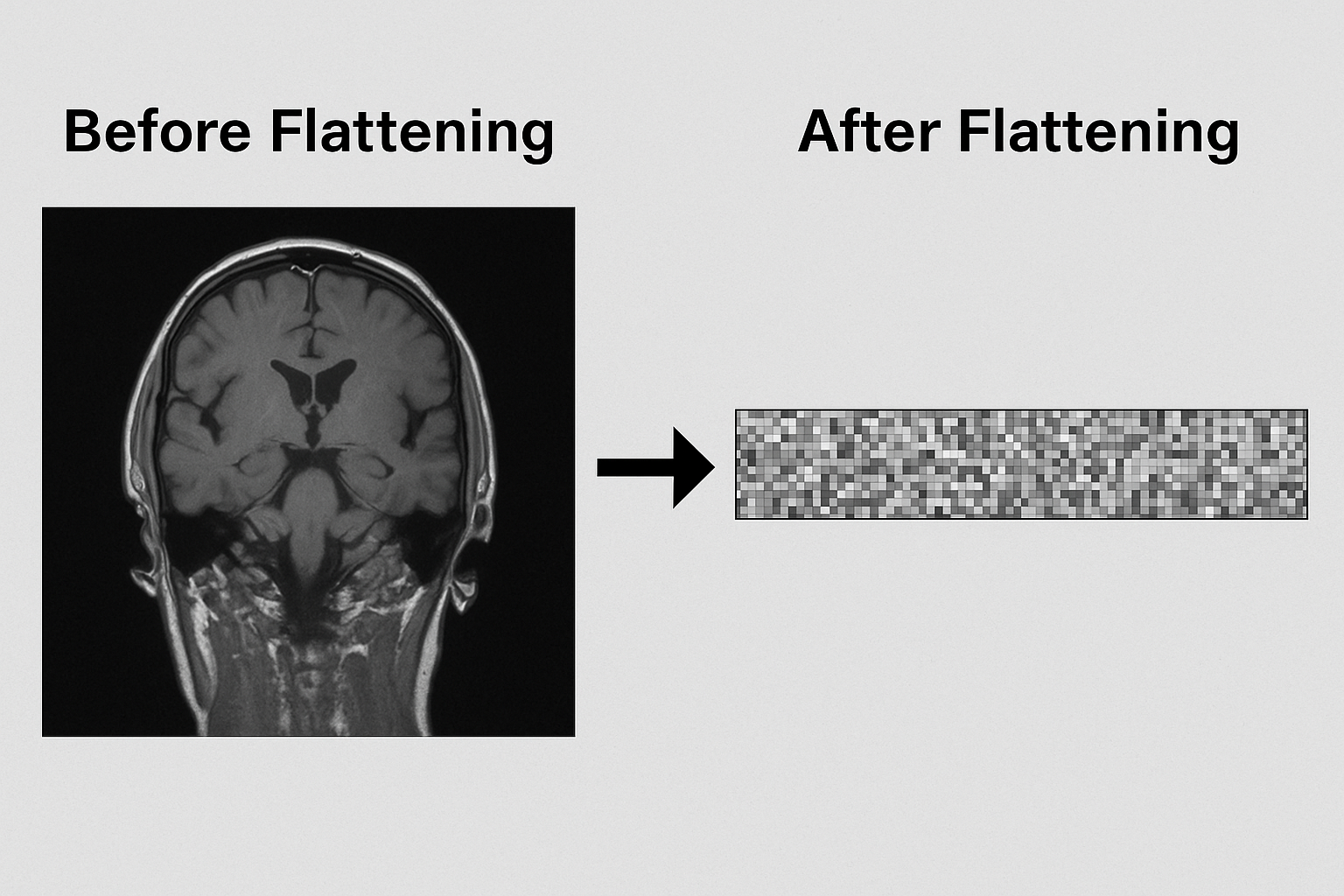
Flattening destroys local relationships

That’s where CNNs shine:

Local connectivity: Filters look at small patches (receptive fields)
Parameter sharing: The same kernel slides across the image
Hierarchical learning: From simple edges to complex organs

Core CNN Operations (2D Example)

Let's break down the key operations that make CNNs so powerful for spatial data:

1. Convolution: The Pattern Detector

            # Typical 2D convolution in PyTorch/Keras
            conv_layer = Conv2D(filters=32, 
                             kernel_size=(3,3), 
                             strides=1, 
                             padding='same')
        

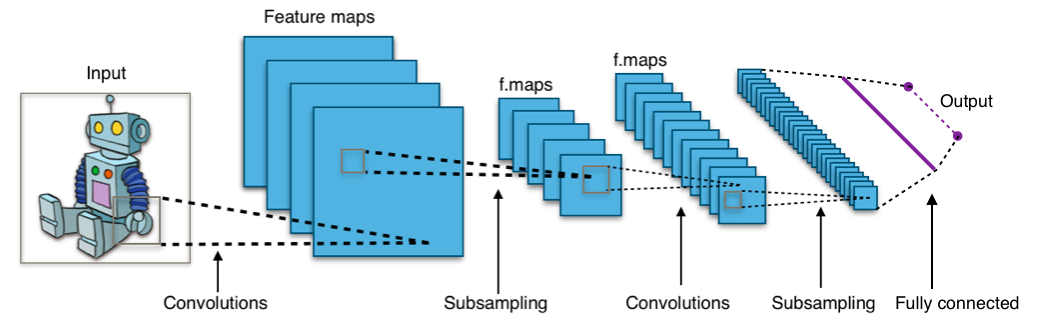
Three-layer CNN architecture showing feature map evolution

What happens: A 3×3 kernel slides across the image, computing dot products at each position
Why it matters: Learns local features like edges, textures, or medical anomalies
Key parameters:
- Filters: Number of feature detectors (32 here)
- Kernel size: Receptive field (3×3 is standard)
- Stride: How many pixels to shift (1=high resolution)

2. Pooling: The Information Compressor

            # Max pooling reduces spatial dimensions
            pool_layer = MaxPool2D(pool_size=(2,2), 
                                strides=2)
        

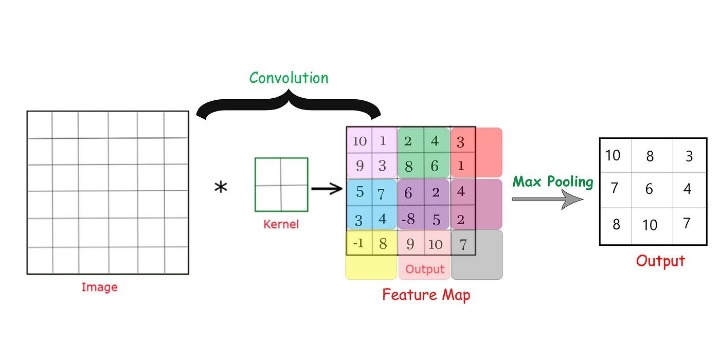
Max pooling operation preserving strongest activations

What happens: Downsamples feature maps by taking maximum values in 2×2 windows
Why it matters:
- Makes network invariant to small translations
- Reduces computational load
- Expands receptive field without adding parameters
Medical imaging tip: Sometimes use average pooling for smoother feature maps

3. Activation: The Non-Linear Transformer

                # ReLU activation (standard for CNNs)
                activation = ReLU()  
                # or LeakyReLU(alpha=0.1) for medical data
            

Mathematically: max(0, x) - zeros out negative activations
Why ReLU?:
- Mitigates vanishing gradients
- Computationally efficient
- Encourages sparse activations (helpful for localized medical features)
Medical variant: LeakyReLU often works better for ECG/EEG data

Putting It All Together

A typical CNN block for medical imaging:

Sequential(
Conv2D(64, (3,3), padding='same'),  # Feature extraction
BatchNormalization(),  # Stabilizes training
ReLU(),
MaxPool2D((2,2)),  # Dimensionality reduction
Dropout(0.2)  # Regularization
)

💡

Pro Tip: For medical images, we often use smaller strides (1 instead of 2) in early layers to preserve fine diagnostic details that might indicate early-stage pathology.

From Pixels to Pulses: CNNs for 1D Signals

What if I told you the same magic behind facial recognition also helps decode heart rhythms? While CNNs were born in the image world, their DNA works just as well for 1D signals like ECGs.

Think about it: An ECG is like a one-dimensional image. Local waveform patterns like P-waves and QRS complexes hold crucial information—exactly the kind of features CNNs are good at extracting.

1D Convolution for ECG Analysis

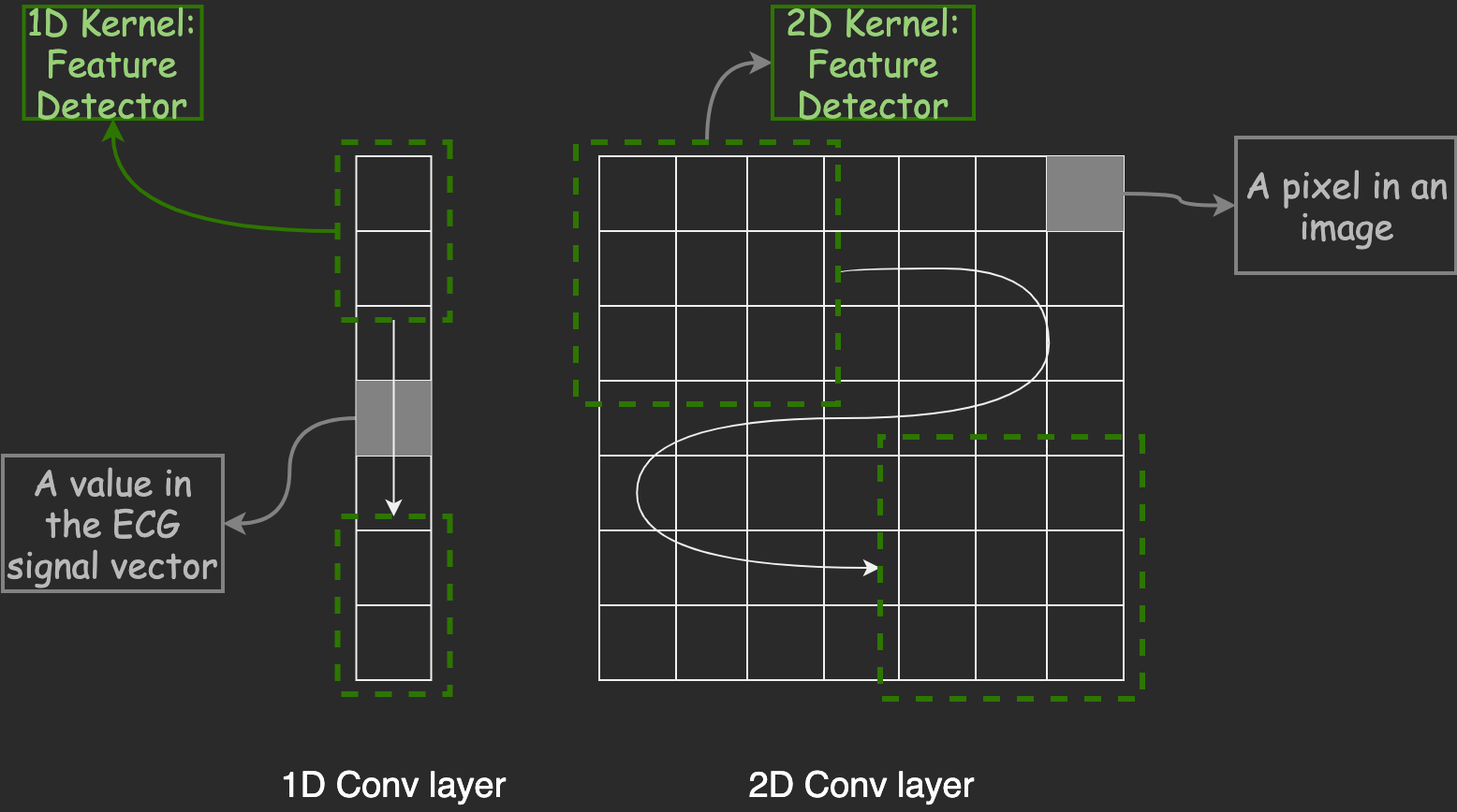
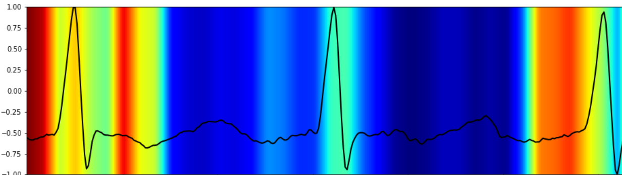
CNN kernels sliding over ECG signals to detect QRS complexes—just like detecting edges in images

    # 1D vs 2D convolution comparison
    # 2D (images)              # 1D (ECG)
    Conv2D(32, (3,3))         Conv1D(32, 3)
    Input: (256,256,3)         Input: (1000,1)  # 1000 samples

Case Study: Cleaning Noisy ECGs with CNNs + Attention

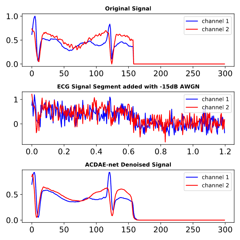
In one of my recent research projects, we developed a hybrid deep learning model called the Attention-Based Convolutional Denoising Autoencoder (ACDAE). Our mission: Clean up highly noisy two-lead ECG signals and accurately detect arrhythmias, even under extreme real-world noise conditions.

The ACDAE architecture blends the strengths of convolutional autoencoders and attention mechanisms:

Encoder: 1D convolutional layers extract compressed, noise-resilient features from raw ECG signals.
Skip Connections: Direct links between encoder and decoder layers help recover fine-grained cardiac signal details lost during downsampling.
Decoder: 1D transposed convolutional layers reconstruct the clean ECG signals from compressed features.
Attention (ECA Module): An efficient channel attention mechanism dynamically focuses on the most diagnostically relevant parts of the signal during reconstruction and classification.

1. Noise Robustness

The denoising autoencoder filters out movement artifacts and high-frequency noise, ensuring that clinical features (like P and T waves) remain intact for accurate diagnosis.

2. Attention Mechanism

Attention gates learn to prioritize signal segments with clinical significance—such as an ST-segment elevation—enhancing interpretability and model trust.

We evaluated ACDAE across four major ECG databases and under varying noise levels from -20 dB to +20 dB SNR. The model achieved impressive results:

19.07 dB average SNR improvement (even under extreme noise).
98.88% arrhythmia classification accuracy with attention-enhanced features.
Lightweight enough for potential deployment on wearable healthcare devices.

Under the Hood:

Encoder: Stacked 1D Conv layers with Leaky ReLU activations
Attention Bottleneck: Efficient Channel Attention (ECA) modules to highlight important cardiac features
Decoder: 1D Transposed Conv layers reconstruct the clean signal
Classifier: A compact fully-connected path for atrial fibrillation (AF) detection

Read the full IEEE paper

Practical Tips: Images vs Signals

Medical signals behave differently from natural images. Here's a cheat sheet I always keep in mind:

Factor	Natural Images	Medical Signals (e.g. ECG)
Augmentation	Flip, rotate freely	Use time-warping, scaling only
Kernel Size	Typically 3×3	Depends on waveform duration (e.g., QRS ≈ 120ms)

Takeaway: The CNN Mindset

Whether I’m analyzing X-rays or heartbeats, my approach remains the same:

Look locally: Slide filters to extract small patterns
Go deep: Stack layers to build abstraction
Tune wisely: Adapt kernel shapes to the data’s domain

CNNs are no longer just for selfies or cat videos—they’re helping diagnose heart disease, detect tumors, and even enhance driver safety. And as we adapt them to new domains, their impact only grows.

Thanks for reading! Feel free to connect if you're working on AI in healthcare—I’d love to learn from your journey too.